DKE Student Projects

Student(s): Enrique Barrueco Mikelarena, Jan Kunnen, Guus Eijsvogels, Maxime Duchateau, Georgios Koutidis, Francesca Battipaglia;
Supervisor(s): Prof. Gerhard Weiss;
Semester: 2020-2021;

Problem statement and motivation:

Dynamic pricing is the concept of a vendor, retailer or other organization that sells products or services adjusting its selling price according to some sort of decision functions in order to reach an objective – e.g. maximizing profit or revenue. Based on a different set of input factors the price the consumer has to pay changes. The big question is how to set the prices such that the aimed objectives are reached as optimal as possible.

A simple example of a market that is subjected to dynamic pricing is the market of airline tickets. Another example is the pricing strategies of world-leading e-commerce provider Amazon (Chen, Mislove, & Wilson, 2016).

A large amount of literature applies the techniques in the field of automated dynamic pricing to a very specific market. The model we want to present tries to address the lack of a general model, that can be used in every type of market. Of course, this can be hard due to the different characteristics of different markets, but some sort of generalization should be possible.

According to Forbes dynamic pricing is “the secret weapon market leaders in different domains of business use to reach their success”. Dynamic pricing however is complex. It is a result from a system that incorporates both a complex demand function and supply function that influence each other, which are also influenced by a lot of internal and external factors on its own (Bitran & Caldentey, 2003). Moreover, the difficulty of implementing a dynamic pricing model is related to the scarce data availability. Due to strategic reasons, firms are not eager to share the information.

Markov Decision Process

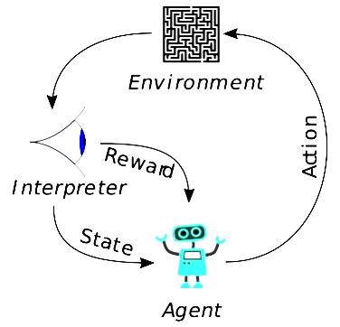
The price learning process can be expressed as a Markov Decision process. The latter involves the definition of a State space, which, in our case, represents the historical data throughout the time horizon. The place where the agent starts its learning process represents the Initial state. In order to move from one state to another, the agent can choose from a definite set of actions, which determine the Action space. All the state-action pairs define the model environment. To each state-action pair is related a reward, that is the expected outcome while following a specific policy.

Markov decision processes are dynamic and, for this reason, they can be used to define optimal prices, which, in turn, are dynamic throughout the time.

Research questions/hypotheses:

• Which is the best definition of a Markov process in this field?
• Which parameters influence the demand function most?
• What is the effect of data scarcity on the efficiency of the model?
• Primary goal: Which model is the most efficient?

Main outcomes:

The main outcomes of the project so far have been:

1. Creating our own dataset scraping data from AliExpress and Alibaba websites. The dataset will be published online and can be used for other reaserches.
2. Definition of demand and cost functions. In this way it is possibile to determine the profit related to different prices and the related demand.

The planned future outcomes are:

1. A fully expanded dataset. This means that more parameters will be taken into account and, hence, the model will be more realistic.
2. Implementation of different Q-learning models.
3. Comparison between the models’ efficiency. In this way is possible too see which of the methods performs better on that specific task.
4. Creation of automated dynamic pricing model. The final model will be able to propose the best price, given the parameters considered and the performance indicator we want to optimize.
5. Generalization performance of dynamic pricing model. The model should be applicable to different kinds of markets, regardless the specific characteristics of each market.

References:

Chen, L., Mislove, A., & Wilson, C. (2016). An empirical analysis of algorithmic pricing on amazon marketplace. In Proceedings of the 25th international conference on world wide web (p. 1339–1349). Republic and Canton of Geneva, CHE: International World Wide Web Conferences Steering Committee. Retrieved from https://doi.org/10.1145/2872427.2883089 doi: 10.1145/2872427.2883089

Bitran, G., & Caldentey, R. (2003, Summer). An overview of pricing models for revenue management. Manufacturing Service Operations Management, 5(3), 203. Retrieved from https:// search-proquest-com.dianus.libr.tue.nl/docview/200628820?accountid=27128

Figures references:

https://en.wikipedia.org/wiki/Reinforcement_learning#/media/File:Reinforcement_learning_diagram.svg

https://www.forbes.com/sites/forbestechcouncil/2019/01/08/dynamic-pricing-the-secret-weapon-used-by-the-worlds-most-successful-companies/

Student(s): Julia Hindel, Mehrdad Pouyanfar, Olivia Kirk, Lucy Quirant, Felix Rustemeyer, Marius Sommerfeld;
Supervisor(s): Rachel Cavill, Katerina Staňková, and Esther Baena (Cancer Research UK);
Semester: 2020-2021.

Problem statement and motivation:

Game theory uses mathematical models to look at how different agents (in this case cells) interact. It is used in many domains, including to re-examine cancer treatment in an innovative way. Doctors tend to treat tumours with medication or radiation until the treatment stops working. This can result in creating more dangerous tumours that have become robust against treatment (Cunningham et al., 2018). Using game theory can help improve patient survival and quality of life (Staňková et al., 2019). We want to predict which treatment works, therefore cell types and their proportions need to be identified.

The aim of this project is to identify cells and establish their proportions. To disentangle/ identify cell mixtures in prostate cancer, two types of data are used. The data is publicly available and comes from The Cancer Genome Atlas (TCGA) database. The first type of data is images of tumour cuts that will be investigated with the help of algorithms which examine cell features (CellProfiler) and group these features together (cluster them). The images are stained with chemicals (in this case H&E staining) which dye the centre of the cell (called cell nucleus) in purple. The software CellProfiler can detect the nucleus size and shape from the stain in the image (Carpenter et al., 2006). Features can be used to establish groups based on similarity, also called hierarchical clustering (Nielsen, 2016). An algorithm clusters extracted features into groups with similar features, e.g. cells with a round nucleus or nucleus diameter of less than 10 μm. Thereby, the algorithm selects the features used for clustering itself without human interaction. The established groups hopefully correspond to cell types. This will then lead to cell identification and cell quantification.

The second type of data is gene expression and methylation data, also called omics data, which will be analysed with various clustering methods called non-negative matrix factorisation (NMF) methods. Genes can be imagined as an instruction manual for what your body looks like and how it is run and are found in the nucleus of every cell of the body. Methylation tells us whether genes are switched on or off. If a gene is switched off, it has no effect on the behaviour of the cell. As there is no labelled data available, gene and methylation data will first be simulated with known cell types. The NMF algorithm takes an input matrix V (e.g. gene expression data) and factorises it into two matrices W and H. In this process, it clusters the columns of input data V (Lee & Seung, 2001; Brunet et al., 2004). NMF can be extended to use multiple inputs (e.g. gene expression and methylation data) simultaneously which is then called joint non-negative matrix factorisation (JNMF). After clustering with (J)NMF, hopefully cell types can be identified and cell proportions quantified (Chalise & Fridley, 2017). There is some uncertainty whether the clusters found correspond to biologically relevant cell types.

Research questions/hypotheses:

• How effective is an NMF-based approach in determining cell proportions from both gene-expression and methylation data?
• How effective is the clustering based on the features extracted from the H&E stained tumour-cut data?
• What hinders and enables effective clustering of cell types within cell mixtures?

Main outcomes:

• Image data: A pipeline using the biology oriented computer vision software ‘CellProfiler’ is fitted to produce a dataset of extracted features from H&E stained tumour-cut data. Furthermore, a hierarchical clustering model can be trained on the extracted features to distinguish different cell types. For every unique cluster, an image that contains a high proportion of that cluster to provide to an expert for aassignment of clusters to ground-truth biology cell types (identification of the clusters).
• Simulation of gene expression & methylation data: In order to test, verify, and gain confidence in the deconvolution algorithms we need to simulate the data with labels. Therefore, we want to deliver a Python script, which is able to simulate data that meets our expectations of reality and resembles the real data.
• Model to identify cell types in gene expression & methylation data: Gene expression and methylation data will be analysed with different variants of non-negative matrix factorisation algorithms. We are going to deliver the method and tuned parameters that performed the best in our experiments.
• Combination of results (if time allows):If good results are obtained from the two outlined approaches, how the pair of results compare and contrast can then be discussed and investigated.

Acknowledgement:

The data used for this research is in whole or partly based upon data generated by the TCGA Research Network: https://www.cancer.gov/tcga

References:

Brunet, J.-P., Tamayo, P., Golub, T. R., & Mesirov, J. P. (2004). Metagenes and molecular pattern discovery using matrix factorization. Proceedings of the National Academy of Sciences, 101(12), 4164–4169. https://doi.org/10.1073/pnas.0308531101

Carpenter, A. E., Jones, T. R., Lamprecht, M. R., Clarke, C., Kang, I., Friman, O., … Sabatini, D. M. (2006). Genome Biology, 7(10), R100. https://doi.org/10.1186/gb-2006-7-10-r100

Chalise, P., & Fridley, B. L. (2017). Integrative clustering of multi-level ‘omic data based on non-negative matrix factorization algorithm. PLOS ONE, 12(5), e0176278.https://doi.org/10.1371/journal.pone.0176278

Cunningham, J. J., Brown, J. S., Gatenby, R. A., & Staňková, K. (2018). Optimal control to develop therapeutic strategies for metastatic castrate resistant prostate cancer. Journal of Theoretical Biology, 459, 67–78.https://doi.org/10.1016/j.jtbi.2018.09.022

Lee, D. D., & Seung, H. S. (2001). Algorithms for non-negative matrix factorization. In Advances in Neural Information Processing Systems 13 – Proceedings of the 2000 Conference, NIPS 2000 (Advances in Neural Information Processing Systems). Neural information processing systems foundation.

McQuin, C., Goodman, A., Chernyshev, V., Kamentsky, L., Cimini, B. A., Karhohs, K. W., … Carpenter, A. E. (2018). CellProfiler 3.0: Next-generation image processing for biology. PLOS Biology, 16(7), e2005970. https://doi.org/10.1371/journal.pbio.2005970

Nielsen, F. (2016). Hierarchical Clustering. In Introduction to HPC with MPI for Data Science (pp. 195–211). Springer International Publishing. https://doi.org/10.1007/978-3-319-21903-5_8

Stanková, K., Brown, J. S., Dalton, W. S., & Gatenby, R. A. (2019). Optimizing Cancer Treatment Using Game Theory. JAMA Oncology, 5(1), 96. https://doi.org/10.1001/jamaoncol.2018.3395

Student(s): Cas Giepmans, Chris du Toit, Kimberly Stessen, Viktor Cef Inselberg, Zsolt Harsányi
Supervisor(s): Cameron Browne & Dennis Soemers
Semester: 2020-2021

Problem statement and motivation:

An important part of designing a new game, is checking whether it is fun and interesting to play. Normally, you test whether the rules are clear, if there’s a lasting interested in playing the game, if losing players can get back on their feet again, and if the majority of matches played end in either wins or losses; not in draws. When a player notices that a match can’t be won anymore, the player might instead want to try to achieve a draw. But what if someone ONLY wants to achieve draws, i.e. has no interest in winning? Well, if the rules of a game don’t account for such intentions, it might be very easy to force a draw whenever a player wants. This is categorized as “non-competitive behaviour”, which is unwanted in basically all competitive games: it often leads to lengthy and boring games that nobody will end up playing. Games that minimize the chance for a draw to occur are called “decisive”, and it is this decisiveness, amongst other things, that we in our project try to measure and quantify.

In a perfect world, every new game would be tested rigorously for its decisiveness through the playing of a large number of matches, between players of different skill levels. Since this kind of testing isn’t always available (but computational resources usually are), testing with Artificial Intelligent players could be a viable alternative. The Ludii General Game System, is a digital framework that has the potential to facilitate this for any and all classic games (board games, card games etc.). Ludii is created for designing, playing, testing and evaluating all kind of games under a single interface. It even has several already implemented AI players that can be used for testing. Currently, Ludii has implementations of over 350 different games. To read more about Ludii, please visit https://ludii.games/index.php.

Every AI player in Ludii is currently configured to try to win. This means that they can be used for regular testing of games, but as described before other “motives” are needed to fully evaluate a game and its characteristics. These “standard” AI players might be so focused on winning, that they overlook secondary strategies which potentially exploit flaws in the game’s design. These strategies could enable a player to never lose, as an example (but also never win). Our goal during this project is to alter these kind of motives of play for the AI players, such that games can be tested reliably. The possible outcomes to any board game are “win”, “loss” and “draw”. On the basis of these outcomes, we can define five different motives of play for AI players. These five variants are:

• Standard: AI tries to win or at least tries to draw (win > draw > loss)
• Defensive: AI tries to avoid defeat (win = draw > loss)
• Blocking: AI tries to draw (win < draw > loss)
• Aggressive: AI only tries to win (win > draw = loss)
• Suicidal: AI tries to lose (win = draw < loss)

Fig. 1: Standard AI Fig. 2: Blocking AI Fig. 3: Suicidal AI

In figure 1 to 3 above you can see some of these AI’s at work. Our AI’s play the circle-team and the size of the blue circles indicate the confidence of the AI to make that move. Figure 1 shows the standard AI which is clearly trying to win. In contrast to the defensive AI in figure 2. This AI is easily able to win, but rather blocks his opponent to avoid defeat. The last AI in figure 3 shows us suicidal behaviour. This AI is in the position to avoid defeat, but rather choses any other move.

Since this is a research project, we will limit our scope of games to 2-player, (alternating) turn-based, “perfect information” games. Perfect information means that there are no hidden elements (like cards in a player’s hand), and both players can observe every part of the game at any point in time. We also limit ourselves to “deterministic” games, meaning that games containing chance-mechanisms won’t be taken into account. While looking into games that fall outside of these definitions is academically interesting, it is better to start with something achievable.

Research questions/hypotheses:

During this project, our main research question that we try to answer is:

• Can we automatically detect rule sets that allow players to avoid defeat at will?

To answer this question, we deconstruct it into several sub-questions around which the project will be structured:

• Can you detect non-competitive behavior in a series of playouts (game logs)?
• Why and how does a rule set not disallow this behavior?
• How can such a rule set be detected automatically for any board game?

Main outcomes:

The ultimate goal of this project is to produce an AI system that can test various board games for robustness. More specifically, we would like to test that in a 2-player board game, one player cannot force a draw (or avoid defeat) at will.

References:

Cameron Browne. Lecture: Automated game design, 2020; Cameron Browne. Ludii general game system.

From student project to news feature: international sci & tech news website The Register covered the #MeToo chatbot prototype that five Data Science for Decision Making master’s students developed together with Jerry Spanakis.

“This tool is part of a bigger project umbrella called SAFE, stemming from Safety Awareness For Empowerment,” Dr Spanakis said. “Our interdisciplinary team’s goal is to improve citizen well-being through prevention, defense, monitoring, and access to resources on sexual harassment and assault.” Read the full article on The Register

 

Furthermore, the chatbot featured in daily newspapers across Europe: the project received attention from El País (Spain), De Morgen (Belgium) and het Financieele Dagblad (the Netherlands, paywalled).

The chatbot received media attention following the preprint release on Arxiv. The paper was be presented during SoGood 2019 – The 4th Workshop on Data Science for Social Good on 20 Sept 2019 – where it is also received the Best Paper Award.

Students: Marcel Böhnen, Maxime Jakubowski, Christian Heil, Zhi Kin Mok, Annika Selbach;
Supervisors: Pieter Collins, Nico Roos;
Semester: 2018-2019.

Fig 1. – What is explainability?

Problem statement and motivation:

What is Machine Learning?

Machine Learning is a subfield of Artificial Intelligence. Unlike normal algorithms where a model is manually programmed to solve a problem, machine learning algorithms use data to learn a model by itself. This model solves a specific task like finding patterns in the data or making predictions. A model takes some input data like, for example, features of some flower: petal width, petal length,… and uses it to predict which type of flower it is.

In terms of interpretability, there are two types of machine learning models: black box models and white box models.

What are black/white box models?

Black box models are complex machine learning models like neural networks or support vector machines. Because of many internal weights and/or parameters black box models cannot be interpreted easily. White box models like linear regression or decision trees are machine learning models that are more interpretable by humans. For example if your algorithm built a decision tree you can look at the tree (if it is not too big) and find the path corresponding to your output and interpret this path of decisions made by the algorithm.

In general, black box models generate much better results than the interpretable white box models. This makes research in black box models more interesting for applications.

Why do we need explainability?

In many domains, simpler, white box models are being used because their predictions are applied to make important decisions. Also, there is the need to be able to verify that their models are working as intended.

Explainability increases user confidence in black box models: when the models are understandable, they are more transparent hence they are more trustworthy. In a setting with potential risk factors, explainability reduces safety concerns as the decisions are comprehensible. Moreover, fair and ethical procedures and results can be ensured when the black box becomes transparent.

In addition, explainability has become essential since a right to explanation is implied by the EU General Data Protection Regulation. So for any business application it is, in fact, a requirement.

Accordingly, more tools to interpret black box models are needed. There are several types of approaches to explain the models. We focus on a type that is called model-agnostic methods.

What do we want to do?

Model-agnostic explanation methods provide an explanation of black box models without looking into them. They only need the input data and output values of a black box to try and explain the predictions it makes.

Since model-agnostic explanation methods are fairly new, we want to experiment with multiple algorithms to make some interpretations of black box models. We make our own implementations of these methods or use existing ones. We alter them and compare them to try and answer the following research questions.

Research questions/hypotheses:

• Which are the existing model-agnostic explainability methods and what are their properties and characteristics?
  We explore five different algorithms and look at what exactly they say about a model. Do they always provide good explanations?
• How do we measure the utility of the generated explanations of each model?
  o For a given domain, is the explanation satisfactory and why?
  How can we determine if the explanations provided by these model-agnostic methods are actually good enough when they are used for some application domains?
• How do the model-agnostic methods perform given different datasets?
  o If the methods performance differs, what is the reason?
  o How can we improve the performance of the method?
  When we use different kind of datasets to train our machine learning method, does this have a big impact on how our methods will perform?

Main Outcomes

Description of the data for the methods

We have a dataset which contains all kinds of features of Iris flowers. It then also contains the name of which type it belongs to. We call one row in this table a data instance.

We trained several machine learning models to predict the flower we are observing by putting in what we know about the sepal length, sepal width, petal length and petal width which we use as features. We can then apply explanation methods on these machine learning models.

Partial Dependence Plots (PDP) and Individual Conditional Expectations (ICE):

PDP’s and ICE’s are plots which display the effect of one feature, like petal width, on the models prediction. When we increase the petal width, we can see the probability of some flower being predicted rise or fall. This is illustrated in figure 2. Every line is for a different flower.

Fig 2. – An example partial dependence plot

 

Accumulated Local Effects (ALE):

ALE’s are similar to the working of PDP’s and ICE’s except that it does not display probabilities but how much of a change there is between predictions.This is called local effects because these changes are calculated by taking intervals of data points instead of going through everything.

Feature Importance:

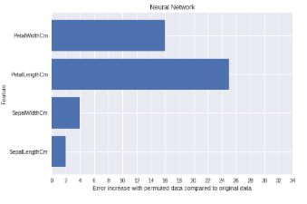
In this method, it is investigated how much the error of the predictions increases when the values for a selected feature of a data instance are shuffled. When the values are shuffled, the information of a feature is incorrect. The higher the increase in error, the more important was that feature for the final prediction. In the example to the left (figure 3), we can see that when the values for the length of the petal (PetalLengthCm) are changed, the prediction error increases by almost 25 percent, indicating that the petal length was important to predict which flower it is. Since the values of the other features are smaller petal length is also the most important feature.

Fig 3. – Plot with the importances of all the features

 

Counterfactual Explanations:

The method explains the black box model by generating data instances opposing to the instance that should be explained. These instances are called counterfactuals. In figure 4, you see an instance of a certain flower type and a corresponding counterfactual which belongs to another flower type. The counterfactual has changed feature values which are the values of a data instance that belongs to the other class. In this case, if the petal length is higher or equal to 2.94, the instance belongs to the flower of type versicolor.

Fig 4. – Example for counterfactuals

To generate counterfactuals the input values of the model are change so that the output of the model gets a new value which is defined before. Also, the distance between the counterfactual and the instance you want to explain should be as short as possible.

In figure 5, you can see an example for a counterfactual. It is the closest data point to the current instance that lies beyond the decision boundary which is described by the model.

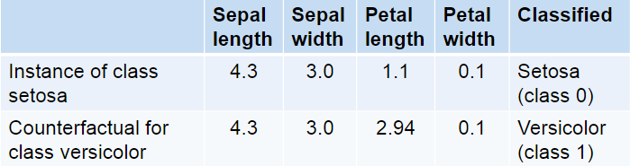
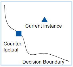
Counterfactuals can be used to get information about how accurate the prediction of the black box model are. Because if the counterfactual is very close to the explained instance, it could be the case that the prediction of the model was wrong. On the other hand, if the distance is big the chance that the model is wrong is very small.

Fig 5. – Example for counterfactuals

 

Future goals

The further goals of this research project would be a comparison between the model-agnostic methods explained before. This would include a description of why they perform well in certain situations and why they would not in others.

Another aspect of this would be the evaluation of what these methods actually say about the machine learning models: what is their expressional power in terms of explainability? A programming library would be provided where all our investigated methods are available and implemented. Finally, we would like to discuss our own view on the utility of these methods for practical use.

References:

Molnar, C. (2018). Interpretable Machine Learning. Retrieved from https://christophm.github.io/interpretable-ml-book/
Lipton, Z. C. (2018). The Mythos of Model Interpretability. Communications of the ACM, 61(10), 36-43. doi:10.1145/3233231
Kaminski, M. (2018). The Right to Explanation, Explained. doi:10.31228/osf.io/rgeus
Hastie T., Tibshirani R., and Friedman J. (2001). The Elements of Statistical Learning. Springer Series in Statistics Springer New York Inc., New York, NY, USA

Students: Quinton Denman, Maxine Hanrieder, Sebas Higler, Lianne Hufkens, Steffen Schneider;
Supervisor: Cameron Browne;
Semester: 2018-2019.

 

Fig 1. – General image that illustrates overall project. Left: Image of a flower. Center: Mesh rendering of the flower. Right: Celtic knotwork of the flower (this image shows an interpretation of the final result)

Problem statement and motivation:

Celtic knotwork has a deep history dating back to 450AD originating with Celtic tribes (Bain, 1990). It has since developed into an artwork consisting of intricate and elaborate knotworks the style of which can be observed in the pictorial gospels called illuminated manuscripts such as the Book of the Kells (Brown, 1980) or the Lindisfarne Gospels (Backhouse, 1981). The knots consist of one or more looped strands woven together and follow a strict over-under pattern, visible in Figure 1. Celtic knotwork is, more often than not, an element within a larger artwork. It serves to add beauty but also imbues the artwork with the history and beliefs of the Celtic culture, see Figure 2. However, Kaplan (2003) mentions that “At some point after the 9th century the techniques used to create Celtic art were lost”, and further explains that George Bain (Bain, 1951) was responsible for reinventing the artistic techniques necessary to create Celtic designs. This technique was then simplified by Ian Bain (Bain, 1990), inadvertently creating methods resembling an algorithmic approach.

The research conducted will aim to understand and then stretch the limits of two aspects present within the challenge of automatically generating Celtic knotwork: the generation of a mesh from a grayscale or color image, capturing figures, shapes and internal features; applying authentic Celtic knotwork designs to said mesh whilst retaining the input images’ form and features. A challenge for the computer-generated knotwork will be to respect the rules implicitly used by traditional artists, ensuring that designs incorporate imperfections present in human work.

The research is not isolated and could lead to further developments in other fields. For example, the generation of a mesh that captures the internal features of an input image could have other applications in areas such as Robotics and Pattern Recognition. This serves to highlight the broader possibilities evident within the proposed research, stressing that whilst the application is very specific, the methods used to realize procedurally generated Celtic knotwork can be extended into other areas. Furthermore, the introduction of more Celtic knotwork could spread the history and culture to a wider audience.

Fig 2. – Authentic Celtic knotwork from Book of Kells.

Research questions/hypotheses:

The key research challenge in this project will be to generate a mesh from a given image that best captures the figure’s shape and internal features while remaining as regular as possible. Generating the knotwork from this mesh is expected to be comparatively straightforward. The research questions are formulated as follows:

 

• How can a mesh be generated to best capture the figure shapes and internal features of an image, while maximising regularity in the mesh elements?
• How can human-like Celtic knotwork best be generated from said mesh?

Main outcomes:

• The primary outcome of this project is a program that takes an image as input and outputs an image that depicts the input image’s features and shapes in Celtic knotwork style.
• From the input image a mesh generation method forms the basis onto which the knotwork is applied. The generated mesh ideally has a regular arrangment of predominantly quadrilateral elements. Moreover, the mesh’s density is inversly proportional to the intensity of the image (i.e. the mesh is denser in darker areas) to reflect the image’s depth in the knotwork.
• The knotwork adheres to a strict over-under pattern, the threads have some undulation and other attributes to mimic a human’s touch and it contains repeated motifs as found in authentic Celtic knotwork.

References:

Backhouse, J. (1981). The Lindisfarne Gospels . Phaidon Oxford.
Bain, G. (1951). The Methods of Construction of Celtic Art . W. MacLellan.
Bain, I. (1990). Celtic Knotwork . Celtic Interest Series. Constable.
Brown, P. (1980). The Book of Kells . Knopf; 1st American ed edition.
Edelsbrunner, H. (2001). Geometry and topology for mesh generation , volume 7. Cambridge University Press.
Fung, K. (2007). Celtic knot generator. BSc (Hons) thesis, University of Bath.
Gross, J. L. and Tucker, T. W. (2011). A celtic framework for knots and links. Discrete & Computational Geometry, 46(1):86-99. Kaplan, M. and Cohen, E. (2003). Computer generated celtic design. Rendering Techniques, 3:9-19.
Martin, D., Arroyo, G., Rodriguez, A., and Isenberg, T. (2017). A survey of digital stippling. Computers & Graphics, 67:24-44.
Mercat, C. (1997). Les entrelacs des enluminures celtes. Pour la science.
Reimann, D. A. (2012). Modular knots from simply decorated uniform tessella- tions. In Proceedings of ISAMA 2012: Eleventh Interdisciplinary Conference of the International Society of the Arts, Mathematics, and Architecture .
Secord, A. (2002). Weighted voronoi stippling. In Proceedings of the 2nd in- ternational symposium on Non-photorealistic animation and rendering , pages 37-43 ACM.
Son, M., Lee, Y., Kang, H., and Lee, S. (2011). Structure grid for directional stippling. Graphical Models, 73(3):74-87.

References:

• Arntzen, Halvard, and Arne Løkketangen. “A local search heuristic for a university timetabling problem.” nine 1.T2 (2003): T45.
• Rossi-Doria, Olivia. “A local search for the timetabling problem.” Proceedings of the 4th International Conference on the Practice and Theory of Automated Timetabling, PATAT. 2002.
• Müller, Tomáš, Keith Murray, and Stephanie Schluttenhofer. “University course timetabling & student sectioning system.” Space Management and Academic Scheduling, Purdue University (2007).
• Ponnalagu, Karthikeyan, Renuka Sindhgatta Rajan, and Bikram Sengupta. “Automatically generating high quality soa design from business process maps based on specified quality goals.” U.S. Patent Application No. 12/885,870.
Download: report
Categories
Bachelor thesis NSO
Criticality of Tasks within Project Management
Example project with 5 phases and 6 tasks labeledStudent: Ashley Peternella
Supervisor: Dr. Jean Derks
Semester: 2015-2016
• Branzei, R., Ferrari, G., Fragnelli, V., and Tijs, S. (2002). Two approaches to the problem of sharing delay costs in joint projects. Annals of Operational Research, Vol. 109, pp. 359–374.
• Castro, J., Daniel, G., and Tejada, J. (2007). A project game for PERT networks. Operations Research Letters 35, pp. 791–798.
• Elmaghraby, S.E. (2000). On criticality and sensitivity in activity networks. European Journal of Operational Research, Vol. 127, No. 2, pp. 220–238.
• Steiner, G.A. (1969). Top management planning macmillan. Quoted on page 481 of Project Management Handbook, 2nd edition.
• Williams, T. (2003). The contribution of mathematical modelling to the practice of project management. IMA J Management Math, Vol. 14, No. 1, pp. 3–30.
Download: Report
Data analysis Machine Learning Master AI semester project RAI
Topic detection and tracking system
Student(s): Daniel Brüggemann, Yannik Hermey, Carsten Orth, Darius Schneider, Stefan Selzer;
Supervisor(s): Dr. Gerasimos (Jerry) Spanakis;
Semester: 2015-2016;
Fig 1. – Dynamic Topic model with emerging topics on the documents of August and September 1996 from RCV1 Corpus
Fig 2. – NMF topics over time on the documents of Reuters archive 2015
Fig 3. – Dynamic Topic model with emerging topics on the documents of August and September 1996 from RCV1 Corpus
[Blei and Lafferty, 2006] Blei, D. M. and Lafferty, J. D. (2006). Dynamic topic models. In Proceedings of the 23rd International Conference on Machine Learning, ICML ’06, pages 113–120, New York, NY, USA. ACM.
[Blei et al., 2003] Blei, D. M., Ng, A. Y., and Jordan, M. I. (2003). Latent dirichlet allocation. J. Mach. Learn. Res., 3:993–1022.
[Cao et al., 2007] Cao, B., Shen, D., Sun, J.-T., Wang, X., Yang, Q., and Chen, Z. (2007). Detect and track latent factors with online nonnegative matrix factorization. IJCAI, page 2689–2694.
[Lewis et al., 2004] Lewis, D. D., Yang, Y., Rose, T. G., and Li, F. (2004). RCV1: A new benchmark collection for text categorization research. J. Mach. Learn. Res., 5:361–397.
[Saha and Sindhwani, 2012] Saha, A. and Sindhwani, V. (2012). Learning evolving and emerging topics in social media: a dynamic NMF approach with temporal regularization. Proceedings of the fifth ACM international conference on Web search and data mining, page 693–702.
[Tannenbaum et al., 2015] Tannenbaum, M., Fischer, A., and Scholtes, J. C. (2015). Dynamic topic detection and tracking using non-negative matrix factorization.
Downloads:
Final Report
Final Presentation