Students: Marcel Böhnen, Maxime Jakubowski, Christian Heil, Zhi Kin Mok, Annika Selbach;
Supervisors: Pieter Collins, Nico Roos;
Semester: 2018-2019.
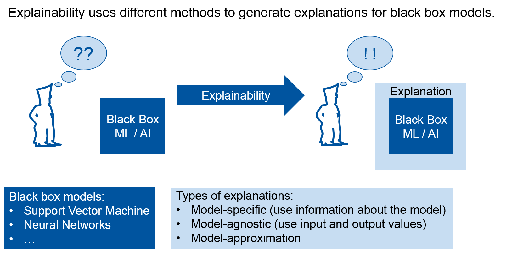
Fig 1. – What is explainability?
Problem statement and motivation:
What is Machine Learning?
Machine Learning is a subfield of Artificial Intelligence. Unlike normal algorithms where a model is manually programmed to solve a problem, machine learning algorithms use data to learn a model by itself. This model solves a specific task like finding patterns in the data or making predictions. A model takes some input data like, for example, features of some flower: petal width, petal length,… and uses it to predict which type of flower it is.
In terms of interpretability, there are two types of machine learning models: black box models and white box models.
What are black/white box models?
Black box models are complex machine learning models like neural networks or support vector machines. Because of many internal weights and/or parameters black box models cannot be interpreted easily. White box models like linear regression or decision trees are machine learning models that are more interpretable by humans. For example if your algorithm built a decision tree you can look at the tree (if it is not too big) and find the path corresponding to your output and interpret this path of decisions made by the algorithm.
In general, black box models generate much better results than the interpretable white box models. This makes research in black box models more interesting for applications.
Why do we need explainability?
In many domains, simpler, white box models are being used because their predictions are applied to make important decisions. Also, there is the need to be able to verify that their models are working as intended.
Explainability increases user confidence in black box models: when the models are understandable, they are more transparent hence they are more trustworthy. In a setting with potential risk factors, explainability reduces safety concerns as the decisions are comprehensible. Moreover, fair and ethical procedures and results can be ensured when the black box becomes transparent.
In addition, explainability has become essential since a right to explanation is implied by the EU General Data Protection Regulation. So for any business application it is, in fact, a requirement.
Accordingly, more tools to interpret black box models are needed. There are several types of approaches to explain the models. We focus on a type that is called model-agnostic methods.
What do we want to do?
Model-agnostic explanation methods provide an explanation of black box models without looking into them. They only need the input data and output values of a black box to try and explain the predictions it makes.
Since model-agnostic explanation methods are fairly new, we want to experiment with multiple algorithms to make some interpretations of black box models. We make our own implementations of these methods or use existing ones. We alter them and compare them to try and answer the following research questions.
Research questions/hypotheses:
- Which are the existing model-agnostic explainability methods and what are their properties and characteristics?
We explore five different algorithms and look at what exactly they say about a model. Do they always provide good explanations? - How do we measure the utility of the generated explanations of each model?
o For a given domain, is the explanation satisfactory and why?
How can we determine if the explanations provided by these model-agnostic methods are actually good enough when they are used for some application domains? - How do the model-agnostic methods perform given different datasets?
o If the methods performance differs, what is the reason?
o How can we improve the performance of the method?
When we use different kind of datasets to train our machine learning method, does this have a big impact on how our methods will perform?
Main Outcomes
Description of the data for the methods
We have a dataset which contains all kinds of features of Iris flowers. It then also contains the name of which type it belongs to. We call one row in this table a data instance.
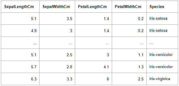
We trained several machine learning models to predict the flower we are observing by putting in what we know about the sepal length, sepal width, petal length and petal width which we use as features. We can then apply explanation methods on these machine learning models.
Partial Dependence Plots (PDP) and Individual Conditional Expectations (ICE):
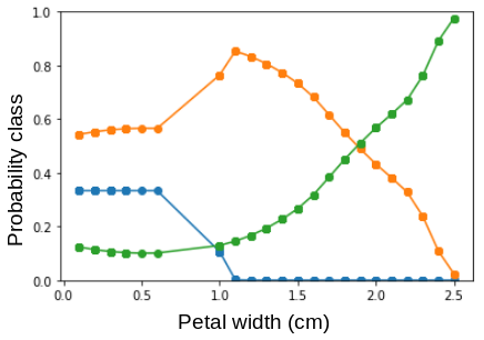
PDP’s and ICE’s are plots which display the effect of one feature, like petal width, on the models prediction. When we increase the petal width, we can see the probability of some flower being predicted rise or fall. This is illustrated in figure 2. Every line is for a different flower.
Fig 2. – An example partial dependence plot
Accumulated Local Effects (ALE):
ALE’s are similar to the working of PDP’s and ICE’s except that it does not display probabilities but how much of a change there is between predictions.This is called local effects because these changes are calculated by taking intervals of data points instead of going through everything.
Feature Importance:
In this method, it is investigated how much the error of the predictions increases when the values for a selected feature of a data instance are shuffled. When the values are shuffled, the information of a feature is incorrect. The higher the increase in error, the more important was that feature for the final prediction. In the example to the left (figure 3), 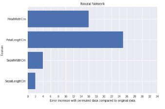 we can see that when the values for the length of the petal (PetalLengthCm) are changed, the prediction error increases by almost 25 percent, indicating that the petal length was important to predict which flower it is. Since the values of the other features are smaller petal length is also the most important feature.
Fig 3. – Plot with the importances of all the features
Counterfactual Explanations:
The method explains the black box model by generating data instances opposing to the instance that should be explained. These instances are called counterfactuals. In figure 4, you see an instance of a certain flower type and a corresponding counterfactual which belongs to another flower type. The counterfactual has changed feature values which are the values of a data instance that belongs to the other class. In this case, if the petal length is higher or equal to 2.94, the instance belongs to the flower of type versicolor.
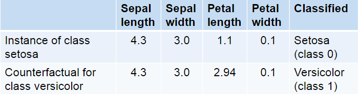
Fig 4. – Example for counterfactuals
To generate counterfactuals the input values of the model are change so that the output of the model gets a new value which is defined before. Also, the distance between the counterfactual and the instance you want to explain should be as short as possible.
In figure 5, you can see an example for a counterfactual. It is the closest data point to the current instance that lies beyond the decision boundary which is described by the model.
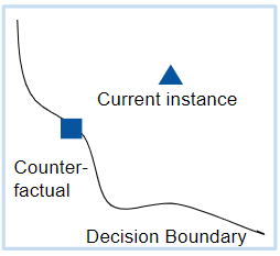 Counterfactuals can be used to get information about how accurate the prediction of the black box model are. Because if the counterfactual is very close to the explained instance, it could be the case that the prediction of the model was wrong. On the other hand, if the distance is big the chance that the model is wrong is very small.
Fig 5. – Example for counterfactuals
Future goals
The further goals of this research project would be a comparison between the model-agnostic methods explained before. This would include a description of why they perform well in certain situations and why they would not in others.
Another aspect of this would be the evaluation of what these methods actually say about the machine learning models: what is their expressional power in terms of explainability? A programming library would be provided where all our investigated methods are available and implemented. Finally, we would like to discuss our own view on the utility of these methods for practical use.
References:
Molnar, C. (2018). Interpretable Machine Learning. Retrieved from https://christophm.github.io/interpretable-ml-book/
Lipton, Z. C. (2018). The Mythos of Model Interpretability. Communications of the ACM, 61(10), 36-43. doi:10.1145/3233231
Kaminski, M. (2018). The Right to Explanation, Explained. doi:10.31228/osf.io/rgeus
Hastie T., Tibshirani R., and Friedman J. (2001). The Elements of Statistical Learning. Springer Series in Statistics Springer New York Inc., New York, NY, USA